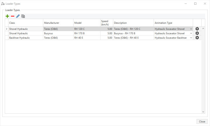
 . The Equipment Library displays.
Click the Animation Type drop-down list to select the animation that suits the equipment. Selecting Custom Type will overwrite the standard animation with your company's animation.
 to the right of the screen to configure operational data.
Loaders can only start a simulation at source locations. Take care to ensure that the source location where the loader is assigned to is also the location where the loader will be for its first task.
Loader types can be duplicated to have their properties modified if needed. To duplicate a loader, select it and click the Copy button on the toolbar. You can rename the equipment if required.
Information about the loader in your haulage system is stored in the equipment library. The information is a combination of local loader characteristics and data from the equipment library. It includes bucket cycle time, bucket payload, loader availability, loading methodology, and operating and capital costs.
Each loader configuration has a link to a loader in the equipment library. The equipment library contains detailed performance characteristics for over 200 loaders. The loader templates apply some of the data from the database as initial values in the configuration.
A lot of the loader information in the loader database is provided for general information only. Of the data that is used, some parameters are used to calculate the default value for the actual bucket payload in the loader template and others are used in loading analysis. If any of this data is missing in the loader database, then default values are assigned:
There are four tabs of data for each loader:
You can add or edit the loader operational data on this tab.
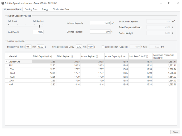
The loader operational data includes:
Bucket passes can be set to either Full Buckets or Full Truck loads by moving the slider. This option is used in the productivity analysis to decide whether or not to put the last bucket load into the truck. As you move the slider, the Last Pass % is updated. You can also enter a value in the Last Pass % field, and the slider will move accordingly.
Each time that the loader places a bucket into the tray of the truck, it checks to make sure that there is enough remaining capacity in the truck. The logic to decide whether or not to add a bucket is shown below.
IF(Remaining Capacity > Bucket Capacity x Last Pass %, Add Bucket, Do Not Add Bucket)
If the aim is to only ever load the truck with full bucket loads, the slider should be to the right (close to the Full Bucket text).
There will be circumstances when the truck requires less than a full bucket load to reach its actual payload. In this case, you can decide that it is better to let the truck travel under-loaded than to waste time with another loader pass. You can set the Last Pass % to determine whether a load will be accepted or rejected as full, as part of the loading methodology (for example, a load of 75% or higher can be considered full).
The full truck strategy assumes that the loader operator will always try to fill the truck, even if the last pass only requires a small portion of a bucket load.
There will be circumstances when the truck requires only a small percentage of a bucket load to reach its actual truck payload. In this case, the decision may be that it is better to let the truck be slightly under-loaded than to waste time with another loader pass to fill the truck.
Alternatively, if the truck requires a large percentage of a bucket load to fill it, the decision may be that it is worth spending the time to put another loader pass in to the truck, so that the truck carries a full load.
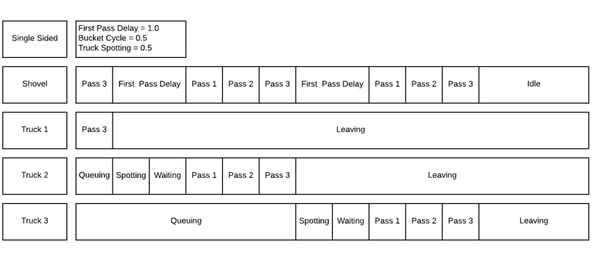
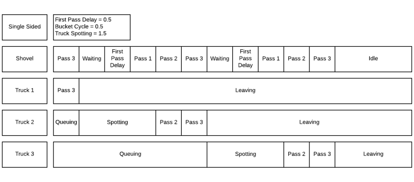
The Bucket Cycle Time field displays the time that it takes the loader to perform one complete load cycle. This includes the loader filling its bucket, manoeuvring to the dump, dumping the bucket load into the truck and manoeuvring to refill the bucket.
The cycle time is specified in minutes or seconds; the other field is automatically calculated. The default cycle time for one bucket is 0.5 minutes.
The first bucket pass delay is the time between when the loader drops the last bucket load into a truck and when it drops the first bucket load into the next truck, minus the average time for one loader pass. Assuming the truck spotting can be coordinated correctly, this represents the time that the loader has its bucket in the air waiting for a truck from the queue. In efficient operations, his time could be zero.
The default value for the first bucket pass delay is zero. To change the default, enter a value in either the minutes or seconds field. The other value is automatically calculated.
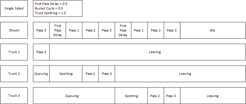
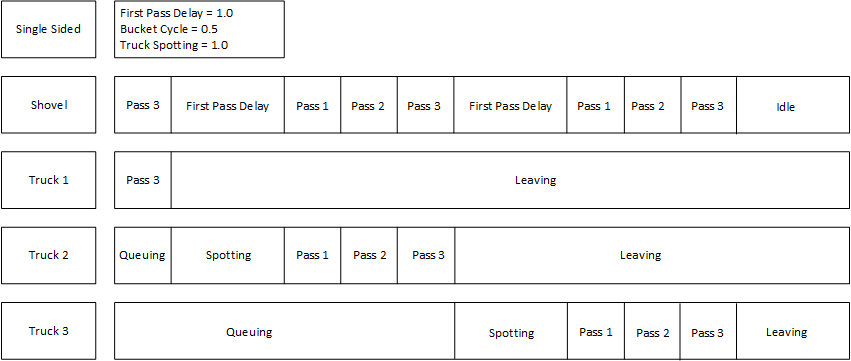
Below are examples of how the Bucket Cycle Time and First Bucket Pass Delay work together to compose the Loading Time.
If a wheel loader is being used to load a truck, additional time is included in the cycle for transport and manoeuvring.
When a wheel loader is acting as a loader, loading a truck, it needs extra time to manoeuvre and transport the load to where the truck is spotted. This extra time can be added using these two fields. The time is added to the wheel loader loading time.
When Surge Loader is selected, there will be an intermediate step between the loading unit and truck. Rather than loading the truck directly, the loader will load the surge loader which will then load the truck.
A surge loader has two configurations; capacity and rate. The capacity is the amount of material that the surge loader can hold when full. The rate is used to calculate the time to load the truck from the surge loader.
Enterprise equipment comes from the Master Equipment Library (MEL). When enterprise equipment is added to the model, more information is shown in the Operational Data tab.
When you first open Equipment Library to add an equipment type to the model, it displays only the enterprise and user (equipment copied to the user library) equipment. An example screenshot is shown below. Notice the filter at the bottom of the screen. Different information is displayed depending on the library type.
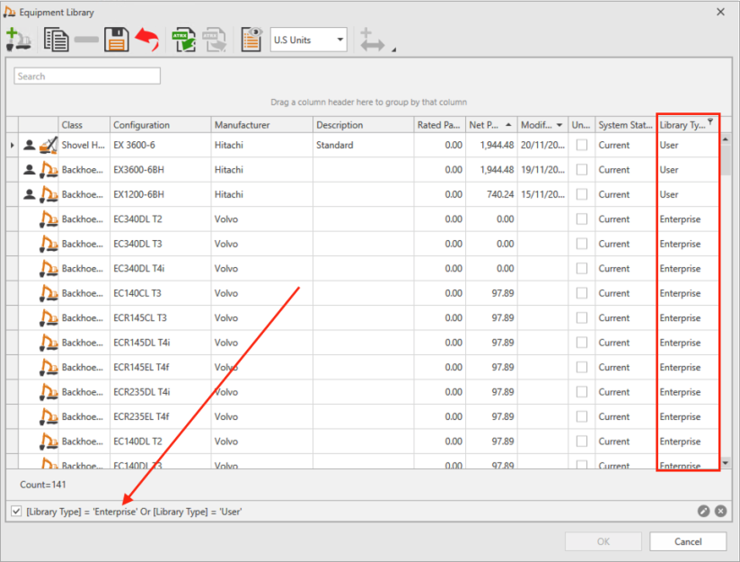
The Save button is only available when editing User equipment. Once you have made your changes, click Save, then click OK at the bottom of the screen.
If you want to see the standard equipment as well, you can either clear the filter check box, or remove it by clicking on the  on the bottom right of the screen. Edit the filter by clicking
  .
.
Extra fields that display for enterprise equipment are Duty Cycle, Operator Skill and Position.
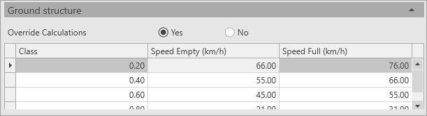
When adding enterprise equipment into the model, the Ground Structure is not editable when the equipment is opened in Equipment Library. This is because enterprise equipment has calculations that modify ground structure speeds based on other selections when configuring the machine.
The Override Calculations check box allows you to override the ground structure speeds. If the check box is selected, the calculation fields under the equipment configuration are greyed out.
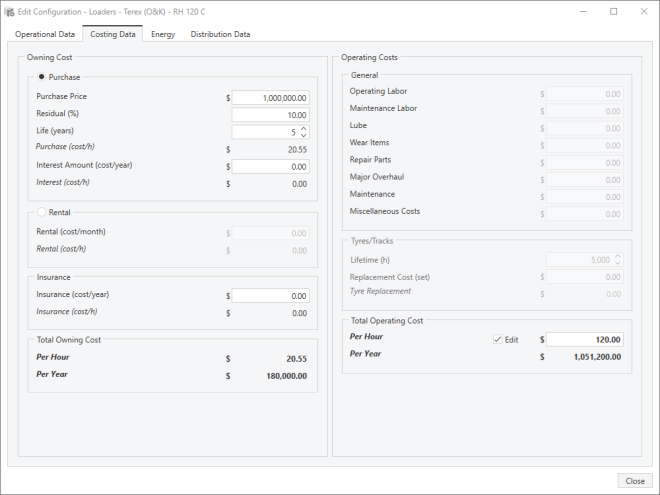
Owning costs are the costs of having the equipment available on-site. Ownership costs accumulate whether or not the equipment is operating. Purchase and rental are both supported ownership cost options. All purchasing costs are converted to an hourly rate, which is then applied to every hour in a calendar year.
Enter the capital cost of the equipment in the Purchase Price field.
Residual percentage is the value of the equipment as a percentage of the purchase price.
The life of the equipment is the time between the purchase of the equipment and the sale of the equipment (at the end of its useful life).
If Rental is selected, it is used instead of purchase price. Insurance costs can be added for both purchase and rental options.
Operating costs for the equipment are specified in dollars per operating hour. The total operating cost is divided into the following categories:
The Tyres/Tracks section is used to calculate the hourly cost of tyres or tracks.

Select Edit to ignore the individual costs and enter the total operating cost.
On this tab, select whether the vehicle is powered by Diesel or Electrical.
Diesel and Electrical screens have the same information.
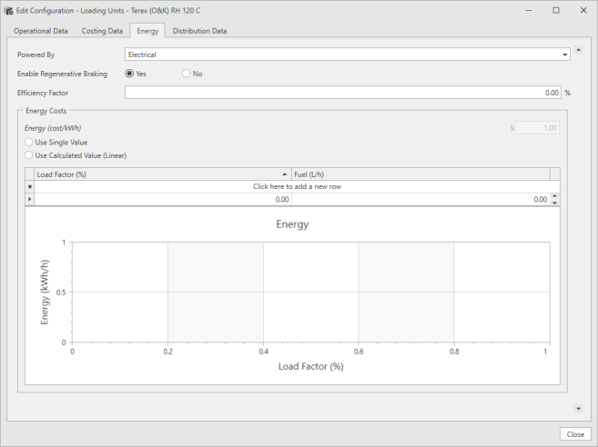
To use a constant energy consumption value for the equipment, select Use Single Value. This value is typically used if fuel usage is based on historic consumption information, and more detailed information is not available. When Use Single Value is selected the curve only shows a line that represents the single fuel usage.
If Use Calculated Value (Linear) is selected, the software uses the fuel calculator and the values are shown in the energy curve. When user-defined fuel is set by selecting the Edit check box, you can edit the Idle and Loading energy consumptions, which are then represented in the curve.
The energy cost changes to reflect the appropriate cost (Diesel or Electrical).
Refer to Energy for more information about energy conversion.
The Energy Curve graph at the bottom of the Energy Costs panel is a simple two-dimensional graphical representation of the energy usage of the selected equipment type. The X axis of the curve represents the load factor which is calculated by the percentage of current and maximum acceleration or deceleration on any road segment. Load factor ranges from -100 to +100. The negative values represent the deceleration, while the positive values represent the acceleration. The Y axis represents the amount of energy used per hour for a given load factor.
Distribution data for the loader is stored for Bucket Cycle Time and Bucket Payload.
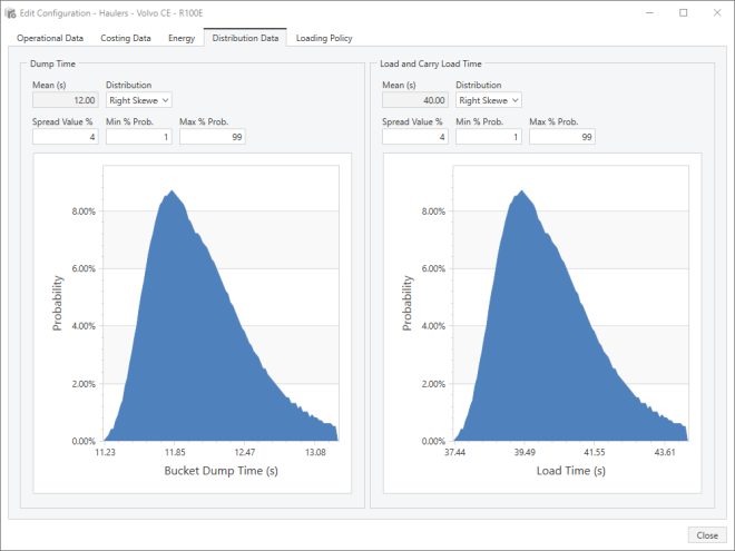
The mean of the distribution is the value for which there is a 50% probability of occurrence. If a deterministic, or fixed value, analysis were being calculated, the variable would have this value.
The mean for each variable is defined on the Operational Data tab in either the bucket cycle time or dumping time field, and cannot be edited from the Distribution Data tab.
There are four standard distribution types provided. The first three standard distributions types are:
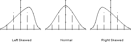
The fourth standard distribution is a uniform distribution, where the variable always has the value of the mean. Select the distribution type you want to use.
The spread value defines how narrow or wide the distribution curve is. If the spread value is small, there will be little variation in the value of the hauler variable. If the spread value is large, there will be a lot of variation in the value of the hauler variable. This is illustrated in the following distribution curves.
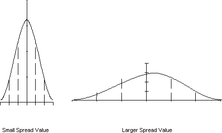
Spread values can be edited and are specified as a percentage above the mean.
The minimum and maximum percentage probability values are used to restrict the range of the selected distribution. The values can be edited and are specified as a percentage of the distribution.